ML Summary Series (2) - Bias-Variance Tradeoff

We are all familiar with the workflow of supervised learning: fit models on training data, and make predictions on the test set. But why should performance of models in the training set tell us anything about that in the test set? Is model performance always generalizable to new data? Learning theory aims to address these questions under a general, abstract formulation of the supervised learning problem, without specifying details like the type of model or the source of data. It also gives a formal explanation of bias-variance tradeoff, one of the most important concepts for prediction. This post, however, will not dive deep into the abstract learning theory, but instead will focus on deriving the bias-variance relationship under a simple example.

We start by an example of curve fitting. Suppose our data points (which are also called “examples”) fall on a 2-dimensional plain.

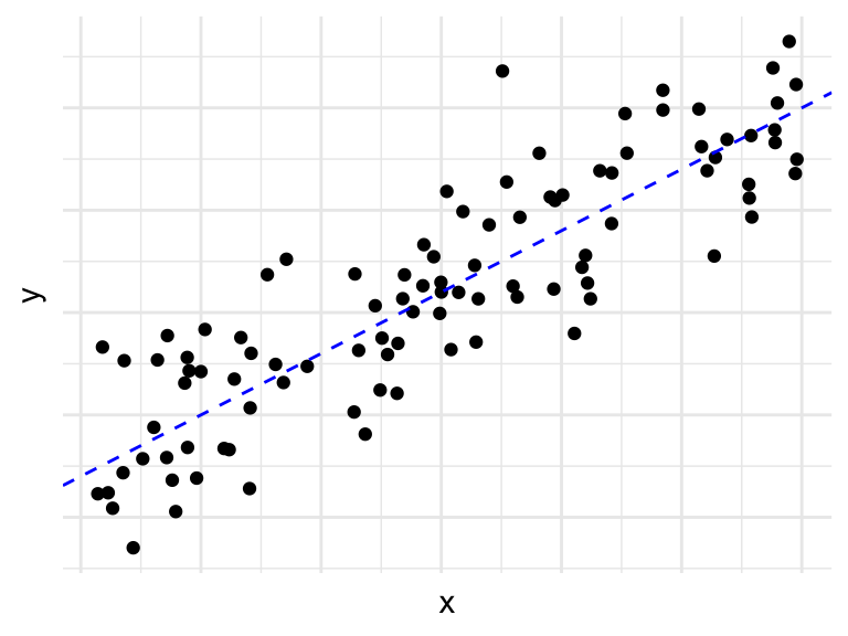
From this visualization, we see that \(y\) may be (linearly) associated with \(x\), and we could potentially use \(x\) to predict \(y\). We use \(f\) to denote the true association between \(x\) and \(y\): \(y=f(x)+\varepsilon\). Note that in real data, there is always going to be some level of noise in \(y\), and therefore, \(y\) will not follow the trend of \(y=f(x)\) exactly. So, although \(f(x)\) is a scalar, we treat \(y\) as a random variable with the component of a normal distributed noise \(\varepsilon \sim N(0, \sigma^2)\).

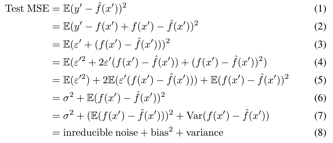
When a machine learning model comes in (I would use linear regression in this case), it tries to learn an approximate of the true association, \(\hat{f}\). Then, when we apply the trained model on new data \(x'\) with the true label \(y'\) unknown, the approximate is used to calculate the prediction: \(\hat{y'} = \hat{f}(x')\). Now, suppose we use mean-squared-error (MSE) to measure the performance of the model. It can be derived that the MSE on new data can be decomposed into three components:

Note that in the above decomposition, we made 2 assumptions:

• Data in the training and the test set need to come from the same distribution. In other words, if we collect data from a data pool to train the model, where the true association is \(f\), then the new data need to be from the same pool with the same association. Of course, if the true association for new data is actually \(g\), which is irrelevant of \(f\), then we are likely not going to make a good prediction.

• All examples should be independent. This is an assumption made by many classic models, and reflects the fact that the underlying association should be invariant of the data collected. If some examples in the data pool are correlated but some are not, then the association behind the correlated examples will be different from that of the uncorrelated ones.

To sum up, in order to make meaningful predictions, we assume that training and test data are independent and identically distributed (i.i.d.).

Under these assumptions, we can now make sense of the derivation. (2) to (3) comes from the assumption of identical distribution, meaning that the true label of the new example can be expressed as \(y' = f(x') + \varepsilon', \varepsilon' \sim N(0, \sigma^2)\). After expanding the squared term from (3) to (5), we use the independent assumption to get (6). Note that in this formation, \(x\) and \(f(x)\) are scalars, but \(\hat{f}\) depends on the entire training set, including the noise in the training data. Therefore, both \(\hat{f}\) and the prediction values \(\hat{f}(x')\) should be seen as random variables. Because the noise in test data, \(\varepsilon'\), and the trained model, \(\hat{f}\), are independent, the interaction term in (5), \(2E(\varepsilon'(f(x') - \hat{f}(x')))\), equals 0. Finally, we use the formula for variance of any random variable to derive (7) from (6): \(var(X) = E(X^2) - (EX)^2\). The decomposition is derived with mean-squared-error measure in curve fitting, but it also generalizes to other data and models.

The term generalization error is used to describe the prediction performance (error rate) on new data, which is a concept corresponding to the training error, or error rate on training data. The decomposition shows that bias and variance are two aspects of the generalization error.

• Bias (\(E(f(x')-\hat{f}(x')) = E(y' - \hat{f}(x'))\)) is the average error between the prediction values and the true labels of new data. It reflects the ability of a model to learn the true association \(f\). If a model has high bias, it means that the algorithm was not able to learn a good approximation of true association \(f\).

• Variance (\(var(f(x') - \hat{f}(x'))\)) is the variance of random variable \(\hat{f}(x')\), over different possible training sets. In other words, if we obtain different training data from the pool with association \(f\), variance is how the model performance would change when training on the newly sampled dataset. If a model has high variance, it means that the model is learning the noise of the training data in addition to the true association.

The two kinds of model behaviors corresponding to bias and variance are therefore called “under-fitting” and “over-fitting”, respectively. We would then be able to take action with regard to each model behavior. If a model is under-fitting, i.e. it is not learning a decent approximation of the true association, we can typically observe poor prediction performance even on training data. Then we need to increase the complexity of the model, like by including more features, so that it better captures the underlying association. If a model is over-fitting, it is fitting too much to the training data and even learning the noise. The model will have great accuracy in training, but on data not used in training, it will have poor performance. We then need to decrease model complexity. The last term in the decomposition, \(\sigma^2\) is the noise in the test data, which there is nothing we can do with. It describes an upper bound of prediction power a model can achieve for this test set.

Finally, we explained the concepts of bias and variance, but have not yet mentioned their trade-off. The mathematical details here are more complicated and depend on assumptions of the models used. So we will not dive in further. But it is worth mentioning that in general, an increase in bias will lead to a decrease in variance, and vice versa.

I would close this post with a summary:

• Assumptions for data in supervised learning: training and test data are i.i.d.
• Generalization error: prediction error of trained model on unseen data
• Bias and variance: two aspects of generalization error, generally move in opposite directions: