ML Summary Series (1) - Concepts

- Supervised / unsupervised learning

Key: labeled or unlabeled data

• 2 types of machine learning tasks
• Supervised learning tasks
  • Work with labeled data - that is, each observation comes with a “value” for the target we hope to predict (called “ground truth”)
  • Examples: regression, classification
• Unsupervised learning
  • Work with unlabeled data - data without associated “ground truth”
  • Examples: clustering, anormaly detection, dimension reduction (PCA, ICA), estimation problem involving latent variables (EM)

- Regression / classification

Key: continuous or discrete target variable

• 2 types of supervised learning problems
• Regression: continuous target
• Classification: discrete target

- Generative / discriminative models

Key: P(X|Y) / P(Y|X)

• Discriminative models - P(Y|X)
  • Directly look for a mapping from predictors \(X\) to target \(Y\)
  • Examples: logistic regression, SVM, decision tree
• Generative models - P(X|Y)
  • Aims to describe the distribution of input data given the labels
  • Examples: Naive Bayes, mixture of Gaussians, HMM

- MLE / MAP estimates

Key: Frequentist VS Bayesian, treat parameters as unknown numbers or random variables

• Estimation: a statistical term for evaluating the value of a parameter based on data
• Both are estimation methods which take different views of the model parameters
• MLE - maximum likelihood estimation
  • Frequentist view
  • Sees parameters as fixed scalars (numbers), only that their values are unknown and need to be inferred from the data
• MAP - maximum a posterior estimation
  • Bayesian view
  • Treats parameters as random variables. It specifies a distribution over the parameters which reflects prior knowledge/belief of the parameters (prior distributions), then adjust the distribution based on data (posterior distribution)

- Parametric / non-parametric models

Key: involves estimating a “fixed-sized parameter” or not

• Not as simple as whether the model involves parameters that need to be learned
• “fixed-sized parameter”: a parameter that no longer change after estimation (the training step).
  • Coefficients in linear or logistic regression are fixed-sized parameters - after learning an estimate of these coefficients, we treat the estimate as fixed, known numbers in prediction. The training set is no longer needed in the prediction step.
• Example for a non-parametric algorithm that involves parameter estimation - locally weighted linear regression
  • Same hypothesis and learning methods (gradient descent) as linear regression
  • Associate each training example with a weight parameter
    • Cost function for gradient descent: \(J(w, \theta) = w^{(i)}(y^{(i)}-\theta^Tx^{(i)})^2\)
    • Weight: \(w^{(i)}=\exp(-\frac{(x^{(i)} - x)^2}{2\tau^2})\), in which \(x\) is the test sample to be predicted. This weight is larger for training examples that are close to the test sample \(x\).
  • The weight parameter \(w^{(i)}\) changes for different test samples. Also, the entire training set is needed at prediction step. Therefore, locally weighted linear regression is a non-parametric model.

- L1 vs L2 regularization

Key: norm used & level of sparsity

• Regularization:
  • Goal: reduce the complexity of models and consequently, reduce the risk of overfitting
  • Reduce the effect size of model parameters, by applying a panelty to parameters in optimization during training
• Apply to different norms of parameters, leading to different degree of sparsity in coefficients:
  • L1: panelize \(|\theta|\) - most of the time, shrink some parameters to zero
  • L2: panelize \(\theta^2\) - size of parameters are shrinked, but most of the time, none are reduced to zero
• Why L1 regularization shrinks parameters to zero but L2 does not?

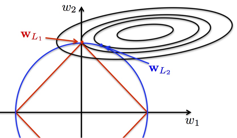
(image is grabbed from here)

Strict theoretical derivation is complicated, but we can use a simple example to understand the intuition. Think of a simple case where we train a linear regression with only 2 parameters: \(y=w_1x_1 + w_2x_2 + \varepsilon\). Denote \(w = (w_1, w_2)^T\). Using the least square method, and adding regularization, the objective function we hope to minimize is

\[min_{w}L(w) + \lambda||w|| = min_{h \geq 0}min_{w, ||w||=h} L(w) + \lambda h\] where \(L(w)\) is the sum of squared error cost function - a quadratic function with regard to parameters \(w_1\) and \(w_2\). \(||*||\) represents the norm, and can be L1 or L2.

The above equation can be translated into the following process: we first constrain the norm of \(w\) as \(h\), and find the minimum of the cost function under the constraint; then we minimize it further with regard to \(h\), which results in the objective function of the regularized least square method.

Constraining \(||w||=h\) means that, for any fixed \(h\), in the parameter space for \(w_1, w_2\), these two parameters can only fall on the lines specified by \(||w||=h\). If we use L1 norm, \(||w||=|w_1| + |w_2| = h\) is diamond-shaped (red); if using L2 norm, \(||w||^2= w_1^2 + w_2^2 = h^2\) is a circle (blue).

In the next step, we hope to find the minimum value for cost function \(L\) given the constraint, i.e. on the lines specified by function \(||w||=h\). \(L\), as we mentioned, is a quadratic function with respect to 2 parameters. It corresponds to a elliptic surface in 3-dimensional space. Finding the minimum then equivalents to looking through the contours of the elliptic surface (the contours are the eclipcses in the image), and see where they intersect with the curve of \(||w||=h\).

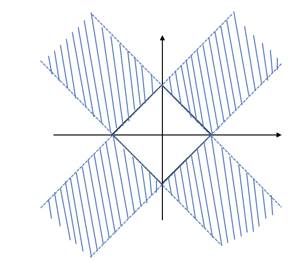
Using L1 norm, it’s more likely that the intersection will happen at the corners (where one of the dimension \(w_1\) or \(w_2\) is 0), than at the edges. If this is not intuitive for you, think of a even simpler case where the contours as circles. The contours will only intersect at edges if the center of the circle is in the shadowed area (image below). When extending the picture to infinity, the shadowed area is just two small stripes on a big canvas. So the probability of that happening is quite small.

On the other hand, when using the L2 norm, intersecting at places where one dimension is 0 is highly unlikely compared to when both \(w_1\) and \(w_2\) are not zeros.

- Under-fitting / over-fitting

Key: decomposition of generalization error of a model (bias-variance tradeoff)

• Assumption of learning algorithms: training and test data are independent, and identically distributed (i.i.d.)
• Generalization error: (in contrary to training error) the error on data not used in training, but come from the same distribution as the training data.
  • Since we make the assumption that training and test data are i.i.d., the model’s generalization error is usually evaluated as the error on test set.
• Bias and variance are two reasons that can lead to high generalization error. In fact, it can be shown that \[ generalization~error = bias + variance + inreducible~noise\] The next post will focus on bias-vairance tradeoff, where I will further explain this decomposition.
• Underfitting:
  • Model has high bias
  • Achieves poor performance even on training set; the model fails to capture the predictor-response association
  • Methods to address: increase model complexity
• Overfitting:
  • Model has high variance
  • Achieves good training performance but poor test set performance; the model fits too well on training data and fails to generalize to other data
  • Methods to address: reduce model complexity (regularization) or add more training data